
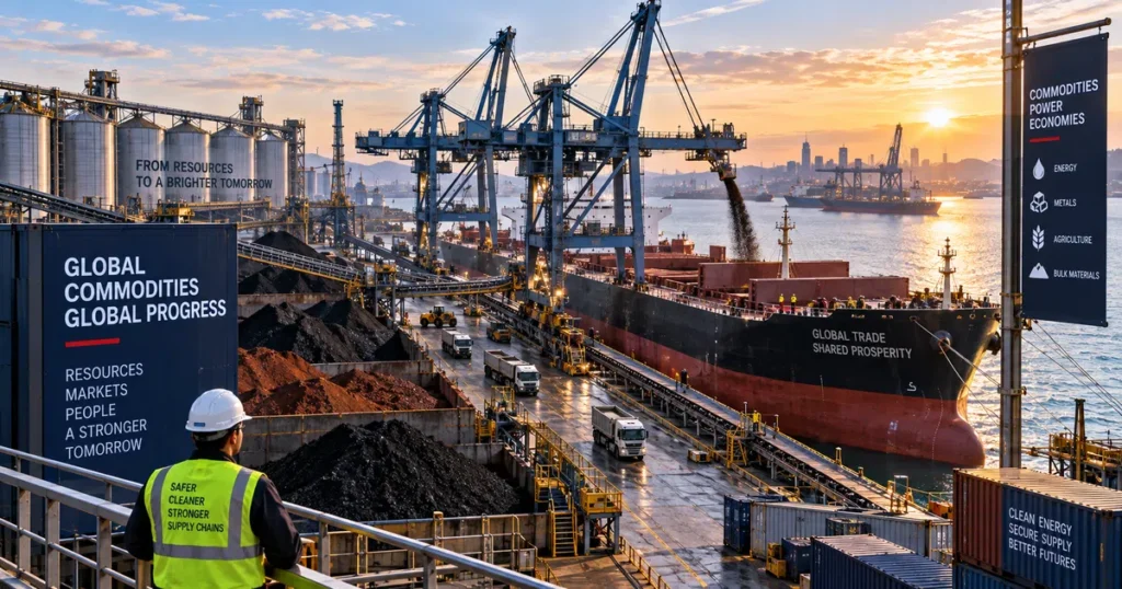
Commodity prices are market prices for raw materials and standardized commodities, formed through the interaction of supply, demand, inventories, production economics, logistics, and market-specific benchmark and pricing mechanisms. Unlike equity shares, whose valuations stem from corporate earnings, management strategy, and discounted future cash flows, raw material valuations reflect the physical balance of extraction, transport logistics, storage friction, and consumption.
Commodity prices are determined primarily by real-world physical supply and demand, but commercial inventories, marginal production economics, weather cycles, geopolitical disruptions, freight bottlenecks, prevailing interest rates, currency fluctuations, and expectations about future market conditions materially influence daily price formation.
Many globally traded raw materials are priced with reference to established regional or international benchmarks, while local cash markets and bilateral transactions may use different pricing mechanisms. Futures and other derivatives prices fluctuate throughout trading sessions, while benchmark or settlement prices are determined according to the methodology and trading rules of the relevant venue, such as the Chicago Mercantile Exchange (CME), the London Metal Exchange (LME), and the Intercontinental Exchange (ICE).
Understanding how commodity prices are established requires examining the microeconomics of marginal production economics, the mathematics of the cost of carry model, the mechanics of futures forward curves (contango and backwardation), the transmission impact of currency valuations, and multi-decade structural price episodes, aligning with the principles detailed in our foundational guide on how stock prices are determined.
What Determines Commodity Prices? Key Factors Affecting Commodity Prices
Quick Answer: How Are Commodity Prices Determined?
Commodity prices are determined primarily by physical supply and demand, inventories, production costs, transportation logistics, weather cycles, geopolitics, and market expectations about future supply-demand balance. For exchange-traded futures contracts, the theoretical relationship between spot and futures prices can be described through the cost-of-carry framework, incorporating financing costs, storage and insurance expenses, and the convenience yield. Over medium to long horizons, prices gravitate toward the marginal cost of production needed to bring sufficient additional supply to market.
Transmission Sequence: Physical Supply/Demand Balance → Commercial Inventories → Reference Benchmarks → Local Cash Basis → Forward Curve Term Structure → Macroeconomic Transmission Channels.
The forces that govern raw material valuations operate across microeconomic, financial, and structural dimensions:
                          ┌──────────────────────────────────────────────┐
                          │         GLOBAL COMMODITY PRICE FORMATION     │
                          └──────────────────────┬───────────────────────┘
                                                 │
         ┌───────────────────────────────────────┴───────────────────────────────────────┐
         │                                                                               │
         ▼                                                                               ▼
┌────────────────────────────────────────┐                     ┌────────────────────────────────────────┐
│ MICROECONOMIC & PHYSICAL FUNDAMENTALS  │                     │ MACROECONOMIC & FINANCIAL DRIVERS      │
├────────────────────────────────────────┤                     ├────────────────────────────────────────┤
│ * Marginal Cost of Extraction Anchor   │                     │ * US Dollar Exchange Rate (Valuation) │
│ * Short-Term Supply/Demand Inelasticity│                     │ * Real Interest Rates (Inventory Carry)│
│ * Physical Storage Capacity & Logistics│                     │ * Global Economic Activity Cycles      │
│ * Weather Anomalies & Biological Cycles│                     │ * Speculative Capital & Risk Premium   │
└───────────────────┬────────────────────┘                     └───────────────────┬────────────────────┘
                    │                                                              │
                    └──────────────────────────────┬───────────────────────────────┘
                                                   │
                                                   ▼
                    ┌─────────────────────────────────────────────────────────────┐
                    │ MARKET PRICE FORMATION: SPOT, CASH & FUTURES RELATIONSHIP   │
                    ├─────────────────────────────────────────────────────────────┤
                    │ * Spot/Cash Market: Price for current or near-term delivery │
                    │   under the relevant market convention                      │
                    │ * Forward Curve: Futures prices across delivery maturities, │
                    │   theoretically anchored by financing, carrying costs,      │
                    │   convenience yield, and market conditions                  │
                    └─────────────────────────────────────────────────────────────┘
The commodity pricing mechanism rests on three core structural realities:
- Extreme Short-Term Price Inelasticity: Consumers cannot instantly stop heating homes or consuming food when prices rise, nor can miners build multi-billion-dollar extraction shafts overnight. This causes physical imbalances to be resolved through sharp pricing adjustments.
- Physical Frictional Constraints: Electronic securities can be stored digitally without carrying costs. Physical commodities require storage, insurance, handling, and transportation, and these carrying costs can influence forward-curve pricing.
- Standardized Reference Pricing: Many raw material markets use standardized grades, specifications, and benchmark prices to facilitate trading, hedging, and physical contract negotiations, as detailed in our guide on what is a commodity. Rather than negotiating individual quality variances, commercial contracts often reference exchange-cleared benchmark grades.
How Commodity Benchmarks Are Established
Quick Answer: How Does a Benchmark Commodity Price Get Established?
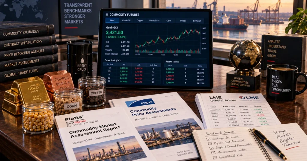
A commodity benchmark or reference price can be established through different market mechanisms. Exchange-traded futures venues publish contract-specific settlement prices under disclosed exchange rules, while physical-market Price Reporting Agencies (PRAs) such as S&P Global Commodity Insights and Argus Media publish assessments using methodologies based on transactions, bids, offers, and other relevant market information.
Benchmark prices solve the problem of market fragmentation. Because raw materials are extracted globally with slight variances in location, quality, and delivery timing, international trade requires common pricing anchors:
| Benchmark Channel | Pricing Methodology & Inputs | Representative Assets | Primary Governing Venues / Bodies |
| Exchange-Traded Derivatives | Standardized contracts traded through exchange matching systems, with contract-specific daily settlement methodologies | NYMEX WTI Crude, CBOT Corn, COMEX Gold, LME Base Metals | CME Group Rulebooks, ICE Operations, London Metal Exchange |
| Assessed Physical Spot (PRAs) | Methodology-based assessments using transactions, bids, offers, and other physical-market information | Dated Brent, Iron Ore 62% Fe CFR China, Jet Fuel Cargoes | S&P Global Platts, Argus Media, Fastmarkets |
- Exchange-Traded Settlement Prices: Venues such as CME and ICE publish official daily settlement prices according to contract-specific methodologies documented in official exchange rulebooks. Depending on the product, these methodologies can use transaction prices, volume-weighted average prices (VWAP) during a defined settlement window, bid/ask information, closing ranges, or other approved market inputs. These published prices can serve as important reference points for bilateral physical contracts, options, and commodity investment products worldwide.
- Physical Over-The-Counter (OTC) Differentials: Physical merchants execute contracts quoted as a “differential” against the benchmark (e.g., Dated Brent + $1.50/bbl or LME Copper Cash – $20/ton). This differential reflects local transportation freight, regional supply-demand balance, and specific chemical purity adjustments.
What Anchors Commodity Prices Over the Long Run? Marginal Cost and Supply Inelasticity
Quick Answer: What Anchors Commodity Prices Over the Long Run?
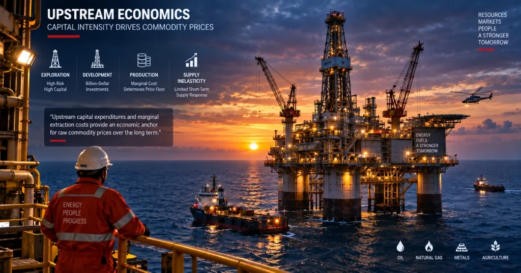
Over medium to long horizons, commodity prices are strongly influenced by the Marginal Cost of Production—the cost required to extract, process, and transport the additional supply needed to satisfy aggregate market demand. Cost curves help illustrate how much production capacity becomes economic at different price levels. If prices remain below operating costs for prolonged periods, high-cost supply is idled or deferred, tightening physical inventories and helping reconnect prices with production economics over time.
Price ($)
  ▲
  │                                                      / (Supply Curve: Highly Inelastic Short-Term)
  │                                                     /
  │                                                    /
  │                         Equilibrium Price         /
  │                                (P*)              /
  ├───────────────────────────────────●─────────────/
  │                                  / \           /
  │                                 /   \         /
  │                                /     \       /
  │                               /       \     /
  │                              /         \   /
  │  Marginal Cost Economic Anchor┌─────────\─/─────────────────────────────
  │                             │            \
  │                             │             \ (Demand Curve: Highly Inelastic Short-Term)
  └─────────────────────────────┴──────────────\────────────────────────────► Quantity (Q)
1. The Mechanics of the Global Cost Curve
Every physical market operates along a ranked supply cost curve (often termed a “cost curve” or “merit order”):
- Tier 1 (Low-Cost Producers): Operators with abundant, easily accessible reserves (such as conventional onshore Middle Eastern crude oil or open-pit Chilean copper mines with high ore grades). These producers boast cash lifting costs well below average global market levels.
- Tier 2 (Mid-Tier Producers): Typical commercial producers requiring standard capital intensity to sustain operations.
- Tier 3 (Marginal Producers): High-cost operators (such as deepwater offshore drillers, low-grade underground miners, or complex oil sands extractors).
When global demand expands, additional supply must be sourced from progressively more costly capacity, spare capacity must be utilized, or new investment must be undertaken. Market-clearing prices can therefore rise enough to make additional or marginal supply economic, while the relevant threshold depends on operating costs, sustaining expenditure, capital requirements, financing conditions, and expectations about future prices. Conversely, during cyclical demand collapses, prices can fall toward levels at which higher-cost production becomes uneconomic, causing some capacity to be idled or investment to be deferred.
2. Supply Inelasticity and Adjustment Dynamics
In manufacturing, supply can often be scaled within weeks. In primary resource extraction, development requires multi-year planning:
- Developing a commercial copper mine requires extended periods of geological surveying, environmental permitting, and heavy civil construction.
- Drilling and completing an ultra-deepwater exploration well requires extensive long-lead engineering.
Because primary supply cannot adjust instantaneously to sudden demand expansions, prices may rise sharply, encouraging demand reduction, substitution, inventory releases, and ultimately new investment in supply.
The Mathematical Engine: Cost of Carry and Forward Curve Pricing
Quick Answer: How Are Commodity Futures Prices Determined?
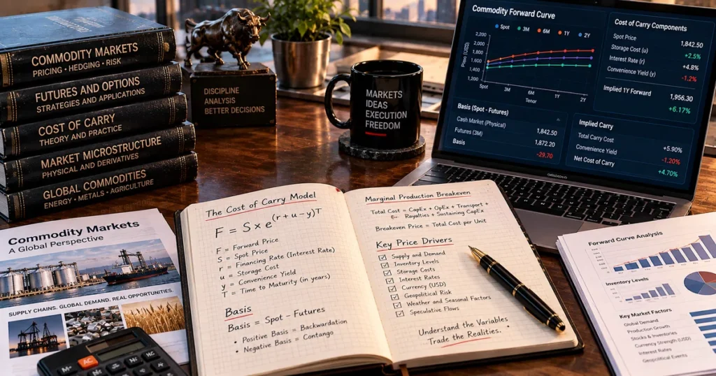
The theoretical forward price relates the current spot price to financing, storage, insurance, and convenience-yield conditions through the Cost of Carry Model. Forward pricing conceptually compounds the spot price by the financing interest rate and physical carrying fees, offset by the Convenience Yield (the operational value of physically holding inventory on hand).
Under continuous compounding, the theoretical forward price $F(t, T)$ for delivery at time $T$ is expressed as:
$$F(t, T) = S(t) \cdot e^{(r + u – y)(T – t)}$$
Where:
- $S(t)$ is the current physical spot price.
- $r$ is the financing rate used in the theoretical pricing framework, commonly represented by a risk-free or benchmark interest rate.
- $u$ is the physical storage, handling, and insurance cost rate.
- $y$ is the Convenience Yield, representing the implicit operational or commercial benefit derived from having physical inventory immediately accessible during supply disruptions.
- $(T – t)$ represents the time duration remaining until delivery.
This is a theoretical no-arbitrage framework. For exchange-traded futures, the same economic relationship provides a useful theoretical benchmark, but actual futures pricing also reflects daily settlement, margining, funding arrangements, contract-specific liquidity, and other market frictions, as documented in educational treatises from the Commodity Futures Trading Commission (CFTC Glossary on Carrying Charges) and CME Group Cost of Carry Research.
Understanding Spot-Futures Basis
In physical commerce, the difference between the local cash spot price and the relevant benchmark futures price is known as the Basis:
$$\text{Basis} = \text{Spot Price} – \text{Futures Price}$$
Using the cash-minus-futures convention adopted in this guide:
- Strengthening Basis: A strengthening basis occurs when local spot prices rise relative to futures. Local supply constraints, unexpected regional processing demand, or transit disruptions can cause the basis to strengthen.
- Weakening Basis: A weakening basis occurs when local cash prices fall relative to futures. Local storage saturation, post-harvest gluts, or freight shortages can widen discounts in local cash markets.
The Geometry of Forward Curves: Contango vs. Backwardation
Quick Answer: What Are Contango and Backwardation?
Contango is a forward-curve structure in which later-dated (deferred) futures contracts trade above nearer-dated contracts. When deferred futures prices also trade above the prevailing spot price, the market is additionally described as trading at a premium to spot, reflecting carrying costs, convenience yields, and broader inventory conditions. Backwardation is an inverted forward-curve structure where later-dated futures contracts trade below nearer-dated contracts (with near-term physical delivery commanding a premium), reflecting immediate physical tightness and elevated convenience value.
The shape of the futures curve is an important factor in how futures-based investors experience returns over extended horizons:
Price ($)
  ▲
  │                                      CONTANGO (Futures > Spot)
  │                                     ┌─────────────────────────
  │                                ┌───┘  Upward-sloping curve:
  │                           ┌───┘       Financing and storage carry
  │                      ┌───┘
  ├─────────────────┬───┘
  │  SPOT PRICE     │
  ├─────────────────┴───┐
  │                      └───┐
  │                           └───┐       BACKWARDATION (Spot > Futures)
  │                                └───┐  Downward-sloping curve:
  │                                     └─────────────────────────
  │                                       Physical tightness / inventory scarcity
  └─────────────────────────────────────────────────────────────────► Time to Expiration
Contango and the Potential Negative Roll Contribution
Contango can occur when deferred futures prices trade higher than nearer-term contracts because carrying costs and other market conditions make deferred delivery more expensive; abundant inventories often reinforce this structure. Under these conditions, commercial storage facilities hold surplus supply, and the market prices in commercial carrying costs ($r + u$).
For a long futures strategy that repeatedly rolls contracts in a contangoed market, rolling can create a negative roll contribution when the expiring contract is sold below the price paid for the next contract:
- The fund sells its lower-priced, expiring front-month contract ($F_{\text{front}}$).
- It purchases the more expensive, subsequent delivery contract ($F_{\text{deferred}}$).
- Over multi-year periods, persistent contango can create negative roll yield drag for futures-tracking funds relative to changes in the underlying spot price.
Backwardation and Positive Roll Contributions
Conversely, when an unexpected supply disruption occurs—such as an export embargo, pipeline shutdown, or severe drought—commercial consumers place a high value on having physical inventory immediately available. In theoretical models, this occurs when convenience yield exceeds carrying costs ($y > r + u$).
Under backwardation:
- The cash spot price trades at a premium over deferred contracts.
- A persistent backwardated curve can produce a positive roll contribution for long futures positions, although the effect depends on the contracts being rolled and how the curve changes over time.
- As futures contracts approach expiration, their prices generally converge toward the contract’s relevant cash, spot, or settlement reference, subject to contract specifications, delivery terms, and market frictions.
+---------------------------------------------------------------------------------------------------+
|                                CONTANGO VS. BACKWARDATION COMPARISON                              |
+---------------------+-----------------------------+-----------------------+-----------------------+
| PARAMETER           | CONTANGO (UPWARD-SLOPING)   | BACKWARDATION (INVERTED)| STRUCTURAL IMPLICATION|
+---------------------+-----------------------------+-----------------------+-----------------------+
| **Curve Shape**     | Upward-sloping ($F_1 < F_2$) | Downward-sloping ($F_1 > F_2$)| Describes deferred-   |
|                     |                             |                       | price relationship    |
+---------------------+-----------------------------+-----------------------+-----------------------+
| **Spot vs. Futures**| Spot < Futures Prices       | Spot > Futures Prices | Inventory availability|
+---------------------+-----------------------------+-----------------------+-----------------------+
| **Physical Context**| Deferred supply is priced   | Near-term delivery is | Market balance and    |
|                     | above near-term delivery;   | priced above deferred;| storage incentives    |
|                     | carrying costs contribute   | tight inventories help|                       |
+---------------------+-----------------------------+-----------------------+-----------------------+
| **Convenience Yield**| Carrying costs exceed value | Elevated convenience  | Relative holding cost |
|                     |                             | value / tight physical|                       |
+---------------------+-----------------------------+-----------------------+-----------------------+
| **Roll Contribution**| **Can create negative drag**| **Can generate positive| Impact on rolling funds|
|                     |                             | contribution**        |                       |
+---------------------+-----------------------------+-----------------------+-----------------------+
Macroeconomic Drivers: Currency Fluctuations, Real Rates, and Liquidity

Quick Answer: What Macro Forces Move Commodity Prices?
Important macroeconomic influences on raw material prices include the US Dollar, real interest rates, global economic activity, and financial conditions. Their importance varies across commodities and market regimes. Because many major internationally traded benchmarks are quoted in US Dollars, movements in the dollar create an immediate currency translation effect across international consuming nations.
                      ┌─────────────────────────────────────────┐
                      │    MACRO TRANSMISSION CHANNELS TO RAW   │
                      │               COMMODITIES               │
                      └────────────────────┬────────────────────┘
                                           │
         ┌─────────────────────────────────┴─────────────────────────────────┐
         │                                                                   │
         ▼                                                                   ▼
┌──────────────────────────────────┐               ┌──────────────────────────────────┐
│ MONETARY & CURRENCY FORCES       │               │ REAL-WORLD DEMAND & SUPPLY       │
├──────────────────────────────────┤               ├──────────────────────────────────┤
│ * US Dollar Relationship:        │               │ * Global Industrial Output:      │
│   All else equal, dollar swings  │               │   Manufacturing expansion drives │
│   impact foreign buying power    │   base metals and energy usage   │
│ * Real Interest Rates:           │ * Supply Shocks & Logistics:     │
│   Influence carrying costs and   │   Transit bottlenecks and trade  │
│   physical inventory financing   │   dislocations                   │
└───────────────────┬──────────────┘               └──────────────────┬───────────────┘
                    │                                                 │
                    └────────────────────────┬────────────────────────┘
                                             │
                                             ▼
                    ┌─────────────────────────────────────────────────┐
                    │ AGGREGATE COMMODITY PRICE FORMATION             │
                    └─────────────────────────────────────────────────┘
1. The US Dollar Relationship
Because many major international benchmarks are quoted in US Dollars (USD):
- When the Dollar Weakens: Changes in the dollar can influence the purchasing power of foreign buyers and therefore affect dollar-denominated prices, all else equal. A weaker dollar can increase foreign purchasing power and support dollar-quoted prices.
- When the Dollar Strengthens: All else equal, a stronger Dollar can exert downward pressure on dollar-quoted market prices by raising local-currency import costs for consuming nations, dynamics analyzed in our research on interest rates and exchange rates.
2. Real Interest Rates and Inventory Financing
Nominal interest rates adjusted for inflation can influence the opportunity cost of holding physical inventories and other assets:
- High Real Interest Rates: Higher real interest rates can increase the financing and opportunity cost of holding inventories and may also weigh on interest-sensitive economic activity. The resulting effect on raw material prices varies by sector and macroeconomic regime.
- Low or Negative Real Interest Rates: Lower real interest rates can reduce the opportunity cost of holding non-yielding assets such as gold, although gold prices are also influenced by currency movements, investment demand, central-bank activity, and broader risk conditions, as examined in our study on fed rate cuts and global liquidity.
How Commodity Prices Are Determined in India: MCX, NCDEX, and Currency Transmission
Quick Answer: How Are Commodity Prices Determined in India?
In India, commodity prices are formed through a combination of international reference prices, domestic supply and demand, currency movements, inventories, taxes and duties, logistics, and contract-specific market mechanisms. Traded primarily on the Multi Commodity Exchange (MCX) and the National Commodity & Derivatives Exchange (NCDEX) under SEBI regulation, domestic futures reflect global price discovery alongside local physical market fundamentals.
India is a major consumer and import market for physical gold, crude oil, vegetable oils, and several industrial base metals. Its domestic price formation operates through an integrated transmission mechanism:
┌───────────────────────────────────┐
│ International Reference Price     │ (e.g., COMEX Gold $/oz, NYMEX Crude $/bbl, LME Copper $/t)
└─────────────────┬─────────────────┘
                  │
                  ▼
┌───────────────────────────────────┐
│ USD/INR Currency Translation      │ (Foreign exchange rate movements directly adjust landed rupee value)
└─────────────────┬─────────────────┘
                  │
                  ▼
┌───────────────────────────────────┐
│ Domestic Physical Market Factors  │ (Import tariffs, customs cess, port logistics, local transport,
└─────────────────┬─────────────────┘  regional premiums/discounts, state taxes, inventory levels)
                  │
                  ▼
┌───────────────────────────────────┐
│ Indian Exchange Price Discovery   │ (MCX & NCDEX contract-specific matching, domestic cash basis,
└───────────────────────────────────┘  and physical delivery/settlement mechanisms under SEBI rules)
- Global Benchmark Transmission on MCX: For internationally traded commodities such as crude oil, gold, silver, and several industrial metals, global benchmark prices and the USD/INR exchange rate exert a strong influence on domestic contracts listed on the Multi Commodity Exchange (MCX). Domestic premiums or discounts, applicable taxes and duties, logistics and port costs, inventories, contract specifications, and regional supply-demand conditions can affect the relationship between Indian market prices and international benchmarks.
- Domestic Agricultural Fundamentals (NCDEX): Agricultural commodities traded on the National Commodity & Derivatives Exchange (NCDEX)—such as chana, jeera, guar seed, and soybean—can be strongly influenced by domestic weather and monsoon conditions, sowing acreage, crop estimates, inventories, government policies such as Minimum Support Prices (MSP) where applicable, import/export measures, and domestic consumption patterns.
- SEBI Regulatory Framework: Commodity derivatives in India operate under the Securities and Exchange Board of India (SEBI), including rules governing margins, position limits, trading, clearing, delivery, settlement, and risk management. Physical-delivery contracts can also involve exchange-specified delivery centres, accredited warehouses, quality standards, and electronic warehouse receipts or related settlement mechanisms where applicable, as detailed in our guide on commodity exchange infrastructure.
Commodity Supercycles: Secular Demand Shifts and Infrastructure Booms
Quick Answer: What Is a Commodity Supercycle?
A commodity supercycle generally refers to an unusually long period of sustained price movements associated with broad structural changes in global demand and supply. Definitions, duration, and the commodities included can vary across research methodologies.
+---------------------------------------------------------------------------------------------------+
|               ILLUSTRATIVE HISTORICAL COMMODITY-BOOM AND SUPERCYCLE EPISODES                      |
+---------------------+-----------------------------+-----------------------+-----------------------+
| ILLUSTRATIVE EPISODE| PRIMARY ECONOMIC CATALYST   | CORE COMMODITIES      | HISTORICAL HORIZON    |
+---------------------+-----------------------------+-----------------------+-----------------------+
| **1. American       | Industrialization of the    | Coal, Iron Ore,       | Late 1890s to         |
| Industrialization** | United States; nationwide   | Copper, Agricultural  | World War I           |
|                     | transcontinental railroads  | Grains                | (c. 1895–1918)        |
+---------------------+-----------------------------+-----------------------+-----------------------+
| **2. Wartime        | Military mobilization and   | Crude Oil, Steel,     | Late 1930s to         |
| Mobilization &      | post-WWII reconstruction of | Aluminum, Base        | Early 1950s           |
| Post-WWII Rebuilding| Europe and Japan            | Metals                | (c. 1938–1953)        |
+---------------------+-----------------------------+-----------------------+-----------------------+
| **3. 1970s Energy & | End of Bretton Woods gold   | Crude Oil, Gold,      | Early 1970s to        |
| Stagflation Era**   | convertibility; OPEC oil    | Silver, Agricultural  | Early 1980s           |
|                     | embargoes and inflation     | Staples               | (c. 1971–1981)        |
+---------------------+-----------------------------+-----------------------+-----------------------+
| **4. The China      | Rapid industrialization,    | Copper, Iron Ore,     | Early 2000s to        |
| Urbanization Boom** | urbanization, trade exp.,   | Thermal Coal, Crude   | Mid-2010s             |
|                     | and capital investment      | Oil, Soybeans         | (c. 2001–2014)        |
+---------------------+-----------------------------+-----------------------+-----------------------+
*Note: These episodes are illustrative rather than a standardized academic chronology. Research on commodity supercycles published by the World Bank uses different datasets, commodity baskets, inflation adjustments, and statistical filtering methods, producing different cycle boundaries.
The Anatomy of a Supercycle
- The Structural Demand Shift: An extended economic transformation begins, such as China’s rapid industrialization, urbanization, trade integration, and infrastructure investment during the 2000s.
- The Capacity Deficit: Prolonged low prices prior to the demand expansion leave mining and energy exploration undercapitalized. Existing production capacity cannot expand fast enough to satisfy rising consumption.
- The Sustained Price Expansion: Raw material prices trade at elevated levels over multi-year periods to balance supply and demand.
- The CapEx Expansion & Supply Rebalancing: Extended high margins induce massive corporate capital expenditures. New resource extraction, refining, and pipeline projects are completed. Once large-scale supply projects enter commercial operation years later, global supply expands, leading to cyclical normalization.
Sector-Specific Price Drivers: Energy, Metals, and Agriculture
Quick Answer: What Unique Factors Drive Energy, Metal, and Crop Prices?
Different commodity sectors respond to distinct microeconomic variables: Energy is governed by production targets, transport chokepoints, and refinery margins; Base Metals respond to construction activity, electrical grid expansions, and manufacturing PMIs; Agricultural Crops depend on biological planting cycles, global weather patterns (such as El Niño), and livestock feed margins.
+---------------------------------------------------------------------------------------------------+
|                         SECTOR-SPECIFIC COMMODITY PRICING VARIABLES                               |
+---------------------+-----------------------------+-----------------------+-----------------------+
| COMMODITY SECTOR    | PRIMARY BENCHMARKS          | DOMINANT MICROECONOMIC| ILLUSTRATIVE MARKET   |
|                     |                             | PRICING VARIABLES     | INDICATOR / METRIC    |
+---------------------+-----------------------------+-----------------------+-----------------------+
| **Petroleum &       | WTI Crude (NYMEX),          | OPEC+ policy targets, | The 3:2:1 Crack Spread|
| Hydrocarbons**      | Brent Crude (ICE),          | refining throughput,  | (Refining margin of   |
|                     | Henry Hub Natural Gas       | transit bottlenecks   | crude into fuels)     |
+---------------------+-----------------------------+-----------------------+-----------------------+
| **Industrial /      | LME Copper Grade A,         | Manufacturing PMIs,   | Treatment & Refining  |
| Base Metals**       | Primary Aluminum, Nickel    | grid electrification, | Charges (TC/RCs) for  |
|                     |                             | construction activity | raw ore smelting      |
+---------------------+-----------------------------+-----------------------+-----------------------+
| **Precious Metals** | COMEX Gold (`GC`),          | Real bond yields,     | Gold-to-Silver Ratio; |
|                     | LBMA Silver, Platinum       | central bank reserves,| Central-Bank &        |
|                     |                             | currency hedging      | Investment Demand     |
+---------------------+-----------------------------+-----------------------+-----------------------+
| **Grains &          | CBOT Corn (`ZC`),           | Weather (droughts),   | The Crush Spread      |
| Agricultural**      | CBOT Soybeans (`ZS`),       | acreage allocations,  | (Margin of soybeans   |
|                     | Milling Wheat               | animal feed demand    | into meal and oil)    |
+---------------------+-----------------------------+-----------------------+-----------------------+
1. The Energy Complex: Production Coordination and Refining Spreads
Energy commodities power global transport and industrial manufacturing:
- The Role of OPEC+: OPEC and participating non-OPEC producers coordinate production policies intended to influence oil-market supply and market balance. Changes in production targets, actual output, and member compliance can affect the global supply cushion.
- The Crack Spread: Petroleum refiners process raw crude into usable transportation fuels. As documented by the U.S. Energy Information Administration (EIA), the 3:2:1 Crack Spread is a simplified measure of the short-term refining margin, approximating the value of two barrels of gasoline and one barrel of distillate produced from three barrels of crude oil. It does not represent a refinery’s complete operating profit because other variable and fixed costs are excluded. When refinery capacity is constrained by maintenance or outages, refined product prices can surge while crude oil prices lag.
2. Base Metals: Electrification and Smelter Capacity
Industrial metals serve as physical inputs for infrastructure and capital goods:
- Copper as an Informal Activity Gauge: Because copper is widely used across electrical, construction, manufacturing, and infrastructure applications, its price is sometimes used by market participants as an informal indicator of industrial activity.
- Treatment and Refining Charges (TC/RCs): Miners pay metallurgical smelters Treatment and Refining Charges to process raw copper concentrate into pure cathode sheets. Falling TC/RCs can indicate tighter availability of copper concentrate relative to smelter demand, providing a useful signal about conditions in the upstream concentrate market. However, TC/RC movements do not by themselves predict the direction of refined copper prices.
3. Agricultural Commodities: Climate Cycles and Crush Margins
Crop pricing is strongly influenced by agronomic seasonality and biological constraints:
- Weather and Climate Patterns: Large-scale climate patterns such as El Niño and La Niña can alter regional weather conditions, sometimes increasing drought, excessive rainfall, or temperature risks in important agricultural regions and affecting expected yields.
- The Crush Spread: Agricultural processors purchase raw soybeans to extract high-protein soybean meal (animal feed) and soybean oil (food ingredient and biofuel feedstock). The soybean Crush Spread represents an indicator of the economic margin from processing soybeans into meal and oil and can influence processor utilization and purchasing decisions.
Microstructure and Price Discovery: Spot Cash Markets vs. Derivatives Exchanges
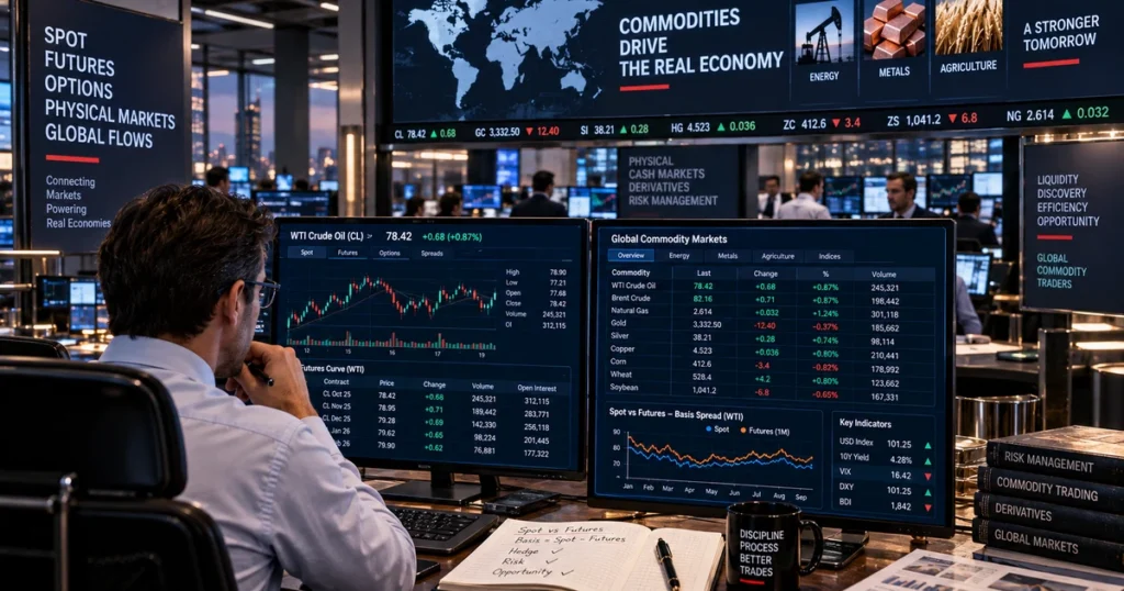
Quick Answer: Where Does Commodity Price Discovery Actually Happen?
For many widely traded commodities, major derivatives exchanges play an important role in benchmark price discovery, while localized physical cash and OTC markets also contribute significantly to price formation. Financial futures markets aggregate substantial order flow to produce continuously updated prices and published settlement prices.
1. The Role of Centralized Derivatives Venues
As detailed in our guide on commodity exchange operations, central clearing associated with many exchange-traded derivatives replaces bilateral counterparty exposure with the clearing house as the central counterparty, subject to the clearing system’s rules and protections:
- Rather than negotiating individual credit terms, participants trade standardized contracts with uniform deliverable grades.
- Electronic matching engines process substantial bids and offers to produce a continuous, publicly transparent price tape.
2. How Physical Deliveries Anchor Derivatives Pricing
Financial derivatives do not trade in complete isolation from the physical economy. For physically deliverable contracts (such as NYMEX WTI crude oil or CME corn), the delivery mechanism provides an important anchor for convergence between futures and physical cash market prices near expiration:
- If a futures contract becomes sufficiently mispriced relative to the deliverable cash market near expiration, arbitrage activity can encourage convergence, subject to delivery costs, quality specifications, location, financing, and other frictions.
- This physical delivery mechanism helps tether derivatives prices to cash market fundamentals upon expiration.
3. Commitments of Traders (COT) and Market Positioning
Published weekly by the Commodity Futures Trading Commission (CFTC), the COT report provides a breakdown of reportable positions based on each Tuesday’s open interest:
- The COT report categorizes traders into groups such as producers/merchants/processors/users, swap dealers, and managed money, allowing analysts to examine changes in aggregate positioning across commercial and non-commercial market participants.
- Positioning extremes may be monitored by some market analysts as a sentiment indicator, but they do not by themselves establish a market reversal or guarantee specific price outcomes.
Comparative Analysis: Commodity Prices vs. Stocks, Bonds, and Real Estate
Quick Answer: How Do Commodity Prices Differ from Traditional Financial Asset Prices?
Physical commodities generally do not generate contractual cash flows such as dividends or coupons; their economic value comes from their physical use, scarcity, expected future prices, and other market factors.
| Dimension / Asset Class | Physical Commodity Prices | Public Equities (Stocks) | Government Bonds | Commercial Real Estate |
| Primary Pricing Framework | Supply-demand balance, marginal economics & cost of carry | Expected earnings/cash flows, valuation multiples & discount rates | Interest rates, expected cash flows & credit considerations | Expected rental income, capitalization rates & property values |
| Cash Flow / Yield | No contractual cash flow; ownership may involve carrying costs and may provide utility or convenience value | Potential dividends and capital appreciation | Contractual coupon payments and principal repayment, subject to credit terms | Rental income and potential capital appreciation |
| Underlying Asset | Physical raw material | Corporate ownership share | Sovereign debt claim | Physical built property |
| Inflation Sensitivity | Often sensitive to inflation through supply costs, demand, currency and monetary conditions | Varies by industry and pricing power | Bond prices generally fall when required yields rise; inflation expectations influence yields | Often influenced by rents, financing costs, and replacement costs |
| Pricing Term Structure | Futures curve (contango/backwardation) | Equity price | Yield curve | Property valuation / capitalization rates |
Understanding these structural differences is essential for investors evaluating commodity-sensitive equity markets such as the Canada TSX and the Australia ASX 200, alongside broader benchmarks like the USA S&P 500.
Common Myths vs. Empirical Facts
- Myth: High commodity prices are created entirely by speculative financial traders.
- Fact: Speculative capital can influence short-term liquidity and price discovery, but commodity prices ultimately reflect the interaction of physical supply, demand, inventories, producers, processors, merchants, consumers, and financial-market participants across the supply chain.
- Myth: A company producing commodities will always see profits surge when commodity prices rise.
- Fact: Extraction companies face operating input-cost inflation (diesel fuel, mining equipment tires, chemical reagents, and specialized engineering labor). If a producer’s operating and capital costs rise at the same rate as the realized commodity market price, corporate profit margins may remain flat.
- Myth: Commodity prices will eventually rise indefinitely because natural resources are finite.
- Fact: High commodity prices stimulate technological innovation, alternative material substitution, and capital investments in exploration. Historically, technological breakthroughs—such as hydraulic fracturing (shale oil) or improved agricultural seed genetics—have shifted supply curves outward, subduing prices for extended periods.
- Myth: Buying a commodity ETF is the same as owning the physical commodity spot price.
- Fact: Many broad commodity exchange-traded products obtain commodity exposure through futures, swaps, or related instruments rather than direct ownership of physical commodities. Futures-based products must roll expiring contracts, so their returns can diverge from changes in the spot price because of roll effects and other costs.
Frequently Asked Questions
What is the simplest explanation of what determines commodity prices?
Commodity prices reflect current and expected future supply, demand, inventories, production economics, and market-specific financial conditions. In the short term, prices respond strongly to available inventories, current production, consumption, transportation constraints, and expectations about near-term supply and demand; over medium to long horizons, prices are strongly influenced by the marginal cost of production needed to satisfy global demand.
What factors affect commodity prices the most?
The primary factors affecting commodity prices include physical supply-demand imbalances, commercial inventory levels, the marginal cost of extraction, US Dollar currency strength, real interest rates, geopolitical transport chokepoints, and weather phenomena affecting agricultural and energy consumption.
What is the difference between spot and futures commodity prices?
Spot commodity prices generally refer to prices for current or near-term physical transactions under the relevant market convention, including specified location, quality, and delivery terms. Futures commodity prices are standardized exchange-traded contract prices. Their theoretical relationship with spot prices can be analyzed using the cost-of-carry framework, while actual prices also reflect market liquidity, funding conditions, contract specifications, expectations, and other market factors.
Why can commodity prices be more volatile than consumer prices?
Many commodities can experience substantial price volatility because primary supply and demand are relatively inelastic in the short run. Consumers cannot instantly stop consuming fuel or food when prices rise, and producers cannot open new mines or drill new fields overnight. Consumer goods also incorporate processing, labor, transportation, and retail margin buffers that can dampen the direct transmission of raw commodity volatility.
How does the US Dollar affect commodity prices?
Because many major international benchmarks are quoted in US Dollars, all else equal, a weakening US Dollar makes commodities relatively cheaper for foreign buyers using other currencies, stimulating global demand and supporting higher dollar-denominated prices. A strengthening dollar conversely makes commodities more expensive internationally, dampening demand.
What does “contango” mean for commodity pricing?
Contango is a forward-curve structure in which later-dated (deferred) futures contracts trade above nearer-dated contracts. When deferred futures prices also trade above the prevailing spot price, the market is additionally described as trading at a premium to spot, reflecting carrying costs, convenience yields, and broader inventory conditions.
What is a commodity supercycle?
A commodity supercycle generally refers to an unusually long period of sustained commodity-price movements associated with broad structural changes in global demand and supply. Definitions, duration, and the commodities included can vary across research methodologies.
Strategic Summary & Core Takeaways
- Physical Economic Reality: Commodity prices reflect the interaction of supply, demand, inventories, production economics, and market-specific quality, location, and delivery conditions across standardized or benchmarked commodity markets.
- The Marginal Cost Anchor: Over medium to long horizons, marginal production economics can act as an important economic anchor, influencing the price levels needed to encourage sufficient additional supply.
- The Cost of Carry Framework: Theoretical forward pricing can be described using the cost-of-carry equation ($F(t, T) = S(t) \cdot e^{(r+u-y)(T-t)}$), incorporating financing costs, physical carrying costs, and convenience yield. Actual futures prices can also reflect margining, liquidity, funding conditions, contract specifications, and other market frictions.
- The Critical Impact of Curve Geometry: Allocators must evaluate the shape of the futures curve; persistent contango can create negative roll yield drag for futures-tracking funds, whereas backwardation can generate positive roll contributions over time.
- Macroeconomic Sensitivity: All else equal, movements in the US Dollar can influence dollar-denominated commodity prices through changes in foreign purchasing power, while real interest rates affect financing costs and the opportunity cost of holding inventories. Global industrial activity and supply conditions remain important commodity-specific drivers.
Next Reading Suggestions
- What Is a Commodity? The Complete Guide to Fungible Goods, Raw Materials, and Global Market Value
- Commodity Exchange: The Complete Guide to Global Trading Hubs, Contract Standardization, and Clearing Mechanics
- What Is Gold? The Complete Guide to Real Money, Store of Value & Why It Matters
- How Stock Prices Are Determined: Market Microstructure, Supply and Demand, and Valuation
- What Is Market Capitalization? The Complete Guide to Market Cap, Company Size, and Valuation
- Interest Rates and Exchange Rates: The Complete Guide to Global Currency Pricing
- Fed Rate Cuts & Global Liquidity: The Complete Guide to Interest Rates, the Fed Balance Sheet, and Asset Markets
- Canada TSX: The Complete Guide to the S&P/TSX Composite Index, Methodology, and Market Structure
- Australia ASX 200: The Complete Guide to the S&P/ASX 200 Index, Methodology, and Market Structure
Author Box & E-E-A-T Verification
Written & Researched By: CurrencyPlans Editorial Research Team
Editorial Review & Methodological Standards: This commodity price educational manual is developed using regulatory statutes, academic microeconomic theory, and primary exchange operating rulebooks. Theoretical pricing frameworks—including the continuous cost of carry model, futures roll yield mechanics, marginal cost curve dynamics, and physical delivery convergence—are informed by official publications and research from the Commodity Futures Trading Commission (CFTC), CME Group, the London Metal Exchange (LME), the Intercontinental Exchange (ICE), the Securities and Exchange Board of India (SEBI), the International Energy Agency (IEA), and the World Bank Commodity Markets Outlook.
Educational References & Market Data Sources
For official futures specifications, historical pricing data, and macroeconomic research, consult primary regulatory and statistical portals directly:
- U.S. Commodity Futures Trading Commission (CFTC Commitments of Traders): CFTC
- CME Group (Commodity Product Specifications & Educational Rulebooks): CME Group
- London Metal Exchange (Non-Ferrous Metals Market Data & Pricing): LME
- Intercontinental Exchange (Global Energy & Benchmark Rules): ICE
- Securities and Exchange Board of India (SEBI Commodity Derivatives Regulations): SEBI
- Multi Commodity Exchange of India (MCX Market Operations & Rules): MCX India
- World Bank (Commodity Markets Outlook & Pink Sheet Data): World Bank
- U.S. Energy Information Administration (Petroleum & Natural Gas Pricing): EIA
- International Energy Agency (Oil Market Reports & Analysis): IEA
Educational Disclaimer
This guide is prepared strictly for educational, research, and informational purposes and does not constitute personalized financial, investment, trading, or tax advice. Commodity spot markets, derivative futures contracts, and natural resource equities carry substantial market and capital risks. Past market pricing patterns and historical futures forward curve shapes do not guarantee future financial returns. Always conduct independent due diligence and consult a licensed fiduciary financial advisor before allocating investment capital.

