
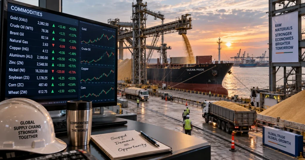
In economics, finance, and capital markets, supply and demand in commodities forms the fundamental mechanism through which global raw material prices are established. While classical microeconomics models market clearing as the intersection of upward-sloping supply and downward-sloping demand curves, the physical architecture of raw material markets introduces distinct structural conditions. Commodities are physical goods governed by subterranean geology, biological crop cycles, multi-year capital investment horizons, regional infrastructure constraints, and storage economics.
Many commodity futures contracts are physically settled, while others are cash-settled against physical benchmark indexes. In physically settled markets, supply, demand, and inventory conditions remain central to price formation. Furthermore, both supply and demand can exhibit pronounced short-run price inelasticity. When an unexpected frost impacts regional agricultural harvests, a labor dispute halts operations at a major copper complex, or an oil pipeline manifold experiences an unscheduled shutdown, physical extraction cannot instantly increase to restore equilibrium. Similarly, commercial transport networks, chemical plants, and electricity generation facilities cannot immediately substitute primary feedstocks without extensive capital re-engineering.
Because short-run supply and demand can be relatively inflexible, modest physical imbalances can produce significant percentage price adjustments across international trading venues, including the Chicago Mercantile Exchange (CME Group), the London Metal Exchange (LME), and the Intercontinental Exchange (ICE). Market participants analyze these dynamics through inventory levels, stocks-to-use ratios, industry cost curves, and forward curve structures, principles directly connected to our foundational analyses of commodity prices and extracted hard commodities.
Executive Summary: The Mechanics of Commodity Market Balance
Quick Answer: How Do Supply and Demand Determine Commodity Prices?
Commodity prices clear where physical production, trade flows, and inventory adjustments balance against industrial, commercial, and retail consumption. Because physical delivery commitments require tangible execution:
- In periods of physical deficit, prices can rise sharply to encourage demand reduction or substitution while drawing down above-ground inventory reserves.
- In periods of physical surplus, prices can decline toward or beneath operating production costs, prompting higher-cost or marginal facilities to curtail output and rebalance the market over time.
                          ┌──────────────────────────────────────────────┐
                          │     THE COMMODITY MARKET BALANCING LEVER     │
                          └──────────────────────┬───────────────────────┘
                                                 │
         ┌───────────────────────────────────────┴───────────────────────────────────────┐
         │                                                                               │
         ▼                                                                               ▼
┌────────────────────────────────────────┐                     ┌────────────────────────────────────────┐
│ PHYSICAL DEFICIT TENDENCIES            │                     │ PHYSICAL SURPLUS TENDENCIES            │
├────────────────────────────────────────┤                     ├────────────────────────────────────────┤
│ * Inventories draw down to low levels  │                     │ * Commercial inventories accumulate    │
│ * Prompt delivery can command premium  │                     │ * Deferred futures can trade above spot│
│ * Forward curve often in BACKWARDATION │                     │ * Forward curve often in CONTANGO      │
│ * Primary Lever: DEMAND CURTAILMENT    │                     │ * Primary Lever: PRODUCTION CURTAILMENT│
│   (Higher prices reduce consumption)   │                     │   (Low prices pressure marginal output)│
└───────────────────┬────────────────────┘                     └───────────────────┬────────────────────┘
                    │                                                              │
                    └──────────────────────────────┬───────────────────────────────┘
                                                   │
                                                   ▼
                    ┌─────────────────────────────────────────────────────────────┐
                    │ EQUILIBRIUM CLEARING MECHANISMS                             │
                    ├─────────────────────────────────────────────────────────────┤
                    │ * Marginal cost of production acts as a long-term reference │
                    │ * Inventory buffers modulate short-term price volatility    │
                    │ * Macroeconomic cycles shape multi-year demand trends       │
                    └─────────────────────────────────────────────────────────────┘
The fundamental properties of commodity supply-demand equilibrium include:
- The Physical Flow Balance: Total commodity production must ultimately be consumed, transformed into secondary products, exported, or absorbed into physical inventory, subject to natural losses and processing yields.
- Short-Run Inelasticity: Neither consumers nor producers can rapidly transform operational infrastructure in response to prompt price movements, requiring market prices to adjust until balance is achieved.
- The Inventory Cushion: Above-ground storage acts as a shock absorber. When stocks are abundant, production or consumption shocks can be cushioned with modest price changes; when inventories are depleted, price sensitivity can become non-linear.
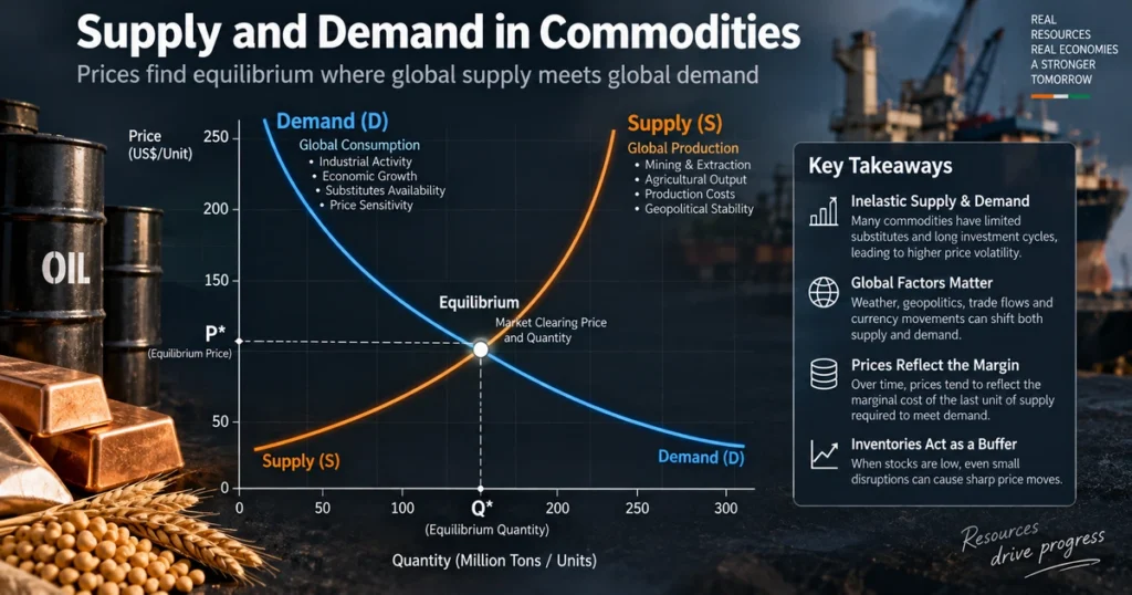
The Classical Model Meets Physical Reality: Steep Inelastic Curves
Quick Answer: What Is Price Elasticity in Commodity Markets?
Price elasticity measures the responsiveness of the quantity supplied or demanded to a change in price. In commodities, both supply and demand can be highly inelastic in the short run. Because short-run supply and demand can be relatively inflexible, even modest physical imbalances can produce disproportionately large price movements, particularly when inventories are low.
                      ┌─────────────────────────────────────────┐
                      │    COMMODITY PRICE INELASTICITY MATRIX  │
                      └────────────────────┬────────────────────┘
                                           │
         ┌─────────────────────────────────┴─────────────────────────────────┐
         │                                                                   │
         ▼                                                                   ▼
┌──────────────────────────────────┐               ┌──────────────────────────────────┐
│ SHORT-RUN HORIZONS               │               │ LONG-RUN HORIZONS                │
├──────────────────────────────────┤               ├──────────────────────────────────┤
│ * Supply: Inelastic              │               │ * Supply: More Elastic           │
│   (Fixed capacity, long lead time│               │   (New mine development, CapEx)  │
│ * Demand: Inelastic              │               │ * Demand: More Elastic           │
│   (Limited immediate substitutes)│               │   (Efficiency gains, substitution│
├──────────────────┬───────────────┘               └──────────────────┬───────────────┘
                   │                                                  │
                   └────────────────────────┬─────────────────────────┘
                                            │
                                            ▼
                   ┌──────────────────────────────────────────────────┐
                   │ NOTE: Illustrative time horizons; actual         │
                   │ adjustment periods vary by commodity and project.│
                   └──────────────────────────────────────────────────┘
1. Why Short-Run Supply Is Often Inelastic
Primary production cannot instantly scale when market prices rise:
- Mining Operations: Commercial metal mines operate within continuous mechanical, safety, and logistical limits. Expanding output requires sinking deeper shafts, constructing additional flotation concentrators, or obtaining environmental permits—processes that routinely involve multi-year capital cycles, as detailed in our guide on hard commodities.
- Agricultural Harvests: Farm crops are bound by agronomic planting and growing seasons. Once planting decisions are made, regional supply is largely set until the next seasonal harvest window, meaning higher prices mid-season cannot immediately generate additional physical grain, as explored in our guide on soft commodities.
- Hydrocarbon Basins: Increasing crude output requires drilling additional wells, building gathering pipelines, and deploying field equipment, which requires operational lead time, as examined in our study on crude oil.
2. Why Short-Run Demand Is Often Inelastic
Commercial and consumer substitution options are constrained over short periods:
- A petroleum refinery cannot readily swap its designated crude assay for another feedstock without altering operational processing yields.
- Industrial manufacturers with established assembly lines cannot immediately substitute alternative metals for copper wiring or aluminum housings without extensive re-engineering and testing.
- Freight transportation fleets and residential heating systems require continuous fuel inputs regardless of immediate market fluctuations.
Because short-run supply and demand curves are steep, shifts in either curve can lead to pronounced price changes before physical quantities adjust.
Supply-Side Drivers: Geology, Capital Cycles, and Extraction Dynamics
Quick Answer: What Primary Factors Drive Commodity Supply?
Commodity supply is influenced by geological deposit characteristics, industry capital investment cycles, operating cash costs, technological adoption, and infrastructure logistics. The lag between initial capital allocation and commercial output frequently drives multi-year cycles in resource availability.
+---------------------------------------------------------------------------------------------------+
|                            PRIMARY COMMODITY SUPPLY DETERMINANTS                                  |
+---------------------+-----------------------------+-----------------------+-----------------------+
| DETERMINANT         | OPERATIONAL MECHANISM       | TIME HORIZON          | MARKET IMPACT         |
+---------------------+-----------------------------+-----------------------+-----------------------+
| **Capital Investment| Multi-year project lead     | Multi-Year Horizon    | Expands or contracts  |
| Cycles**            | times lag price incentives  | (Varies by sector)    | global base capacity  |
+---------------------+-----------------------------+-----------------------+-----------------------+
| **Ore Grade & Basin | Depleting resources require | Structural Horizon    | Raises average energy |
| Depletion**         | greater rock/fluid movement | (Ongoing process)     | and extraction inputs |
+---------------------+-----------------------------+-----------------------+-----------------------+
| **Technological     | Enhanced recovery, seismic  | Multi-Year Horizon    | Lowers unit extraction|
| Innovation**        | modeling, and automation    | (Varies by adoption)  | costs across basins   |
+---------------------+-----------------------------+-----------------------+-----------------------+
| **Operational &     | Strikes, transport outages, | Immediate Horizon     | Generates prompt-month|
| Policy Disruptions**| export bans, and weather    | (Days to months)      | physical supply gaps  |
+---------------------+-----------------------------+-----------------------+-----------------------+
*Note: Illustrative time horizons; actual adjustment periods vary by commodity, jurisdiction, and project complexity.
1. The Capital Investment Cycle
Commodity capacity development typically follows sequential phases:
- Elevated Prices & Project Approvals: Sustained supply deficits generate favorable prices, prompting corporate boards to approve capital investments in new extraction projects.
- Construction and Development Lag: Over subsequent years, capital is deployed to build infrastructure while physical output has not yet reached market, keeping balances relatively tight.
- Capacity Delivery: As multiple large-scale developments enter commercial production simultaneously, market supply expands, potentially creating surpluses if demand growth moderates.
- Market Softening & Capital Discipline: Lower prices compress operating margins, leading producers to defer exploration and curtail greenfield development.
- Depletion & Market Rebalancing: Ongoing depletion gradually absorbs excess production capacity, establishing the conditions for the next cyclical tightening.
2. Resource Depletion and Grade Variation
Over decades of production, highly accessible and high-grade mineral reserves are gradually depleted:
- Many established copper operations now process lower average ore grades than in prior decades, requiring greater material handling, energy, and water per ton of refined metal produced.
- Hydrocarbon extraction increasingly utilizes deepwater offshore reservoirs and tight formations, which require sustained capital investment to maintain baseline production, as detailed in our guide on what is a commodity.
Demand-Side Drivers: Industrialization, Macro Trends, and Seasonality
Quick Answer: What Primary Factors Drive Commodity Demand?
Commodity demand is shaped by global economic output (GDP), manufacturing purchasing managers’ indices (PMI), infrastructure development, currency movements (notably the US Dollar), and seasonal patterns (such as winter heating requirements and post-harvest agricultural consumption).
                          ┌──────────────────────────────────────────────┐
                          │         GLOBAL COMMODITY DEMAND CHANNELS     │
                          └──────────────────────┬───────────────────────┘
                                                 │
         ┌───────────────────────────────────────┴───────────────────────────────────────┐
         │                                                                               │
         ▼                                                                               ▼
┌────────────────────────────────────────┐                     ┌────────────────────────────────────────┐
│ STRUCTURAL & MACROECONOMIC CHANNELS    │                     │ CYCLICAL & SEASONAL CHANNELS           │
├────────────────────────────────────────┤                     ├────────────────────────────────────────┤
│ * Global Industrial Manufacturing PMIs │                     │ * Seasonal Space Heating & Cooling     │
│ * Infrastructure & Urbanization Growth │                     │ * Agricultural Harvest & Field Cycles  │
│ * Energy Transition Electrification    │                     │ * Commercial Transport Peak Seasons    │
│ * US Dollar Exchange Rate Movements    │                     │ * Scheduled Refinery Maintenance Turns │
└───────────────────┬────────────────────┘                     └───────────────────┬────────────────────┘
                    │                                                              │
                    └──────────────────────────────┬───────────────────────────────┘
                                                   │
                                                   ▼
                    ┌─────────────────────────────────────────────────────────────┐
                    │ APPARENT CONSUMPTION & PROCESSING DEMAND                    │
                    └─────────────────────────────────────────────────────────────┘
1. Infrastructure Development and Commodity Intensity
The relationship between economic growth and raw material consumption varies across developmental stages:
- Developed service-oriented economies typically consume lower volumes of raw materials per unit of GDP.
- Developing and emerging economies undergoing significant urbanization and infrastructure build-outs exhibit higher commodity intensity, requiring substantial volumes of structural steel, base metals, concrete, and energy fuels.
- Changes in per-capita income can also drive dietary shifts, increasing demand for protein and animal feed grains, as outlined in our overview of soft commodities.
2. The US Dollar Transmission Channel
Because major international commodity contracts are quoted and cleared in US Dollars:
- When the US Dollar Softens: Dollar-denominated commodities become relatively less expensive in local currencies for non-dollar buyers, which can support international purchasing power and overall demand.
- When the US Dollar Strengthens: Commodities become more expensive in foreign currency terms, which can dampen import demand, as explored in our guide on interest rates and exchange rates.
The Cost Curve Architecture: Cash Costs, AISC, and Marginal Supply
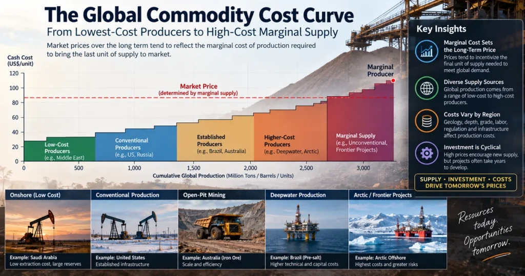
Quick Answer: What Is the Commodity Cost Curve and Why Does It Matter?
A cost curve ranks global production facilities for a specific commodity from lowest to highest cost of production along the horizontal axis against cumulative capacity. Over extended periods, market prices tend to reflect the marginal cost of production—the operating cost of the final production unit required to meet aggregate market demand.
Cost ($/Unit)
  ▲
  │                                                      Higher-Cost Marginal Facilities
  │                                                      ┌──────────────────────────────
  │                                                 ┌────┘ (Complex/Deepwater/Lower-Grade)
  │                                            ┌────┘
  │                                       ┌────┘
  │                                  ┌────┘ Mid-Tier Cost Producers
  │                             ┌────┘      (Standard Commercial Basins)
  │                        ┌────┘
  │                   ┌────┘
  │  Lower-Cost Basins┌┘
  │  (High-Grade/    │
  │   Low-Strip Mine)│
  └──────────────────┴────────────────────────────────────────────────────────► Cumulative Global
                     ◄────────────── Total Market Demand ─────────────►          Production Capacity
                                                                       ▲
                                                                       │
                                                 Price Anchored by Marginal Cost Tier
1. Standardized Industry Cost Classifications
In resource extraction and mining analysis, operating costs are commonly grouped into distinct tiers:
- Cash Operating Costs (C1): Direct on-site operational expenditures, including labor, fuel, power, consumables, and royalties, less byproduct credits.
- All-In Sustaining Costs (AISC): Combines C1 cash costs with sustaining capital expenditures, corporate general and administrative overhead, and site maintenance necessary to maintain current production.
- Incentive Price: The long-term price level required to justify greenfield capital investment, accounting for exploration expenses, development capital, financing costs, and a target return on capital.
2. Cost Curves as Economic Anchors
- Market Expansion: When demand outpaces existing capacity, prices can rise toward or above the long-term incentive price, encouraging capital allocation toward new production assets.
- Market Contraction: When persistent surpluses occur, prices often decline into the upper tiers of the global cost curve. If prices remain below C1 cash operating costs for extended periods, high-cost operations face cash flow pressure, which can prompt operational curtailments that help rebalance physical supply.
The Role of Inventories: Stocks-to-Use Ratios and the Buffer Mechanism
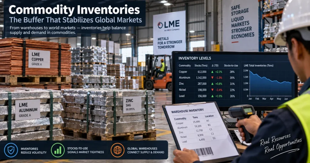
Quick Answer: What Is the Stocks-to-Use Ratio in Commodity Analysis?
The stocks-to-use ratio measures carryover inventory as a percentage of total annual consumption:
$$\text{Stocks-to-Use Ratio} = \frac{\text{Ending Inventories}}{\text{Total Annual Consumption}} \times 100$$
It serves as a benchmark for physical supply cushions. When the ratio is elevated, markets can generally accommodate unexpected disruptions with modest price movement. When the ratio declines toward historically low levels, price sensitivity can increase as physical reserves diminish.
+---------------------------------------------------------------------------------------------------+
|                        INVENTORY CUSHIONS AND MARKET DYNAMICS                                     |
+---------------------+-----------------------------+-----------------------+-----------------------+
| INVENTORY CONTEXT   | BUFFER CHARACTERISTICS      | PRICE IMPLICATIONS    | COMMON SPREAD TENDENCY|
+---------------------+-----------------------------+-----------------------+-----------------------+
| **Elevated Inventory| Substantial carryover stocks| Prices reflect storage| Contango tendencies   |
| Levels**            | provide operational cushion | and carry factors     | (Carry costs active)  |
+---------------------+-----------------------------+-----------------------+-----------------------+
| **Balanced Inventory| Stocks near historical      | Prices reflect ongoing| Flat to moderate      |
| Levels**            | operating averages          | supply-demand trends  | forward spreads       |
+---------------------+-----------------------------+-----------------------+-----------------------+
| **Depleted Inventory| Narrow buffer reserves      | Prices become highly  | Backwardation tend-   |
| Levels**            | increase stock-out risk     | sensitive to shocks   | encies (Prompt premium|
+---------------------+-----------------------------+-----------------------+-----------------------+
*Note: Inventory interpretations and thresholds vary by commodity, storage technology, and trade infrastructure.
1. Non-Linear Price Responses to Low Inventories
Inventory levels influence market sensitivity:
- When physical inventories are abundant, supply outages can often be absorbed by drawing down existing warehouse stocks with muted price reactions.
- When inventories are depleted toward minimum operating levels, identical supply disruptions can lead to significant price reactions as commercial consumers compete for available prompt physical delivery.
2. Visible vs. Invisible Storage
Market analysts monitor two main forms of inventory:
- Visible Stocks: Formally reported, audited inventories held in exchange-monitored facilities, such as LME-approved warehouses, CME delivery points (like Cushing, Oklahoma), and government agricultural balance sheets.
- Invisible (Unreported) Stocks: Privately held inventories located at consumer manufacturing plants, commercial storage terminals, or off-warrant facilities, which can absorb or release volume without appearing in public exchange data.
Anatomy of a Supply Shock: Geopolitics, Weather, and Geological Failures
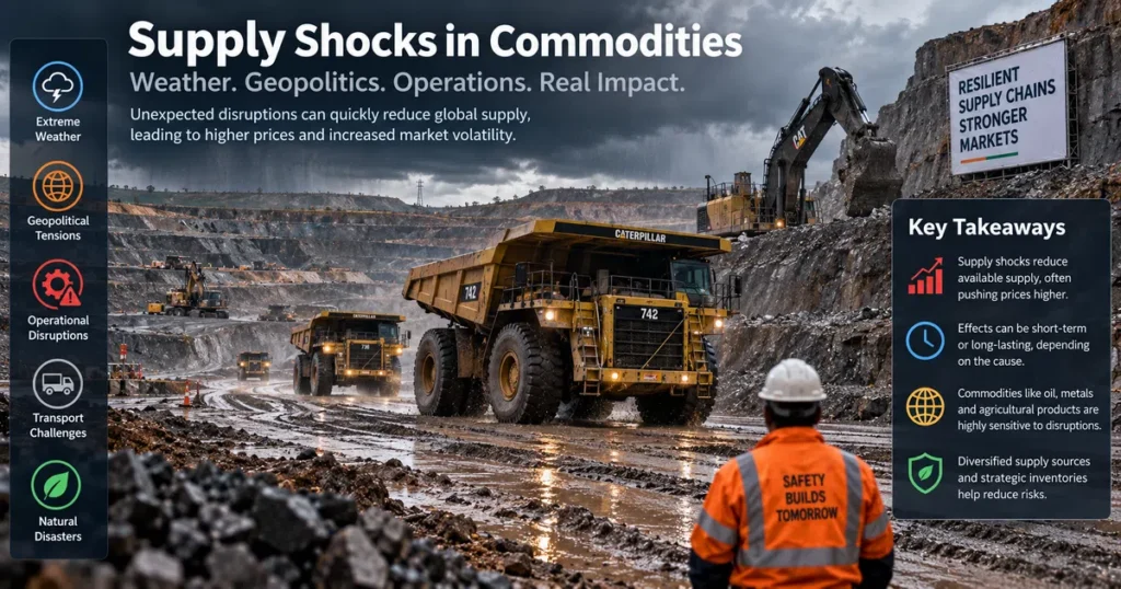
Quick Answer: What Happens During a Commodity Supply Shock?
A supply shock is an unexpected, abrupt decline in available supply caused by exogenous events such as severe weather anomalies, geopolitical trade restrictions, industrial accidents, or natural disasters. Because demand cannot adjust immediately, market prices can rise sharply, shifting prompt prices relative to forward deliveries and encouraging consumers to moderate usage.
                          ┌──────────────────────────────────────────────┐
                          │         ANATOMY OF A SUPPLY SHOCK            │
                          └──────────────────────┬───────────────────────┘
                                                 │
         ┌───────────────────────────────────────┴───────────────────────────────────────┐
         │                                                                               │
         ▼                                                                               ▼
┌────────────────────────────────────────┐                     ┌────────────────────────────────────────┐
│ EXOGENOUS EVENT OCCURS                 │                     │ IMMEDIATE MARKET REACTION              │
├────────────────────────────────────────┤                     ├────────────────────────────────────────┤
│ * Unscheduled export/transit outage    │  ── Prompt ──►      │ * Spot prices can rise sharply relative│
│ * Severe weather anomaly or drought    │     Shortfall       │   to deferred futures contracts        │
│ * Regional facility shutdown or strike │                     │ * Commercial buyers compete for prompt │
│ * Major transport bottleneck           │                     │   physical inventory                   │
└───────────────────┬────────────────────┘                     └───────────────────┬────────────────────┘
                    │                                                              │
                    └──────────────────────────────┬───────────────────────────────┘
                                                   │
                                                   ▼
                    ┌─────────────────────────────────────────────────────────────┐
                    │ REBALANCING PHASE                                           │
                    ├─────────────────────────────────────────────────────────────┤
                    │ * Higher prices encourage conservation, efficiency, or fuel │
                    │   switching where technically feasible                      │
                    │ * Market balance stabilizes as alternative flows mobilize   │
                    └─────────────────────────────────────────────────────────────┘
Case Studies in Market Shocks:
- European Natural Gas Volatility: When regional pipeline supply contracted sharply, European Title Transfer Facility (TTF) benchmark prices reached historic levels. As household heating demand remained essential, price increases led energy-intensive industrial consumers (including fertilizer and primary aluminum plants) to temporarily curtail operations, moderating industrial consumption.
- The 2023/24 Cocoa Supply Disruption: Adverse weather conditions, including unseasonal heavy rainfall followed by intense dry conditions across West Africa (Côte d’Ivoire and Ghana), contributed to the spread of black pod disease and swollen shoot virus. Because West Africa accounts for a major share of global cocoa production, cocoa futures experienced a substantial rally over the crop cycle, leading commercial confectioners to adapt pricing, packaging, and sourcing strategies, as detailed in our guide on soft commodities.
Futures Term Structure: How Contango and Backwardation Signal Physical Balances
Quick Answer: How Do Futures Curves Reflect Supply and Demand?
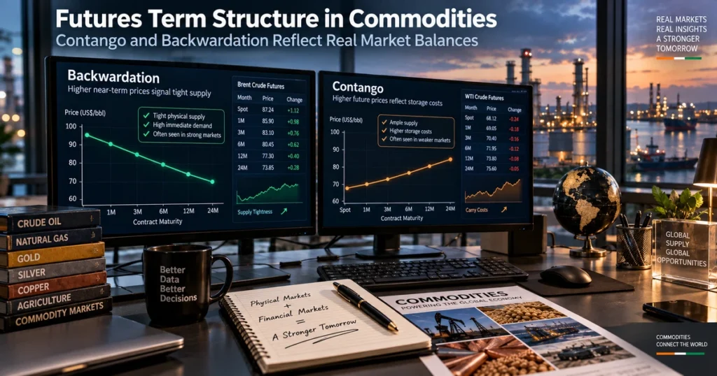
The forward curve reflects market expectations, carrying costs, and immediate physical availability:
- Contango (Upward Sloping): Later-dated contracts trade above near-term contracts ($F > S$). Contango often reflects positive carrying costs (storage, insurance, financing) and/or expectations of higher future prices.
- Backwardation (Downward Sloping): Near-term contracts trade above later-dated contracts ($S > F$). Backwardation can reflect tight prompt supply and a high convenience yield. Neither structure alone proves a physical surplus or deficit.
+---------------------------------------------------------------------------------------------------+
|                        FORWARD CURVE TERM STRUCTURE AND SPREADS                                   |
+---------------------+-----------------------------+-----------------------+-----------------------+
| CURVE STRUCTURE     | ECONOMIC MECHANISM          | DRIVING FORCES        | LONG FUTURES IMPACT   |
+---------------------+-----------------------------+-----------------------+-----------------------+
| **Contango          | Deferred futures trade at   | Storage costs, capital| Long positions rolling|
| (Upward Slope)**    | premium to prompt contracts | financing, expectations| contracts can face   |
|                     | ($F > S$)                   | of future balances    | negative roll yield   |
+---------------------+-----------------------------+-----------------------+-----------------------+
| **Backwardation     | Prompt contracts trade at   | Immediate physical    | Long positions rolling|
| (Downward Slope)**  | premium to deferred contracts| demand, convenience  | contracts can capture |
|                     | ($S > F$)                   | yield, tight buffers  | positive roll yield   |
+---------------------+-----------------------------+-----------------------+-----------------------+
1. The Theory of Storage and the Convenience Yield
The relationship between spot and futures prices is modeled through the Theory of Storage:
$$F_{0,T} = S_0 \times e^{(r + u – y)T}$$
Where:
- $F_{0,T}$ = Futures price for delivery at time $T$
- $S_0$ = Current physical spot price
- $r$ = Financing interest rate
- $u$ = Storage, handling, and insurance cost per unit of time
- $y$ = Convenience Yield (the operational value of physically possessing the commodity)
2. Interpreting Curve Dynamics:
- Low Convenience Yield ($y \approx 0$): When inventories are readily available, physical possession provides minimal operational advantage. Forward prices tend to reflect the costs of storage, financing, and insurance.
- High Convenience Yield ($y > r + u$): When spot supplies are constrained, commercial processors place a significant premium on securing immediate physical deliveries to maintain operations, leading prompt prices to trade above deferred contracts.
The Financialization Factor: Speculators, Hedgers, and Market Clearing
Quick Answer: Do Financial Speculators Distort Commodity Supply and Demand?
Financial market participants—such as commodity trading advisors (CTAs), hedge funds, and institutional allocators—provide trading liquidity and assume price risk from commercial operators. While financial positioning can influence futures pricing and short-term momentum, physical supply, demand, and inventory fundamentals remain central to ultimate market clearing.
                          ┌──────────────────────────────────────────────┐
                          │         COMMODITY PARTICIPANT DYNAMICS       │
                          └──────────────────────┬───────────────────────┘
                                                 │
         ┌───────────────────────────────────────┴───────────────────────────────────────┐
         │                                                                               │
         ▼                                                                               ▼
┌────────────────────────────────────────┐                     ┌────────────────────────────────────────┐
│ COMMERCIAL PARTICIPANTS (HEDGERS)      │                     │ FINANCIAL PARTICIPANTS (SPECULATORS)   │
├────────────────────────────────────────┤                     ├────────────────────────────────────────┤
│ * Mining firms & hydrocarbon drillers  │                     │ * Quantitative Trend-Following CTAs    │
│ * Agricultural producers & processors  │  ── Liquidity ──►   │ * Macro Discretionary Hedge Funds      │
│ * Industrial consumers & manufacturers │     Transfer        │ * Commodity Index Tracker Products     │
├────────────────────────────────────────┤                     ├────────────────────────────────────────┤
│ ROLE: Manage price volatility and      │                     │ ROLE: Provide liquidity and assume     │
│ hedge underlying commercial operations │                     │ price risk in search of returns        │
└────────────────────────────────────────┘                     └────────────────────────────────────────┘
1. Commercial Hedging vs. Speculative Positioning
Market participant data published in the Commitments of Traders (COT) reports by the Commodity Futures Trading Commission (CFTC) illustrates the division of market open interest:
- Commercial Hedgers: Producers and industrial users who trade futures and options to establish forward pricing and manage business margins.
- Financial Allocators: Non-commercial participants who take positions based on macroeconomic trends, quantitative models, and portfolio diversification strategies. Financial participants influence futures pricing and liquidity, while physical market fundamentals establish the baseline for long-term clearing.
2. Physical Delivery and Financial Convergence
Many exchange-traded commodity contracts represent standardized grades or specifications:
- In physically deliverable contracts, the possibility of physical delivery anchors futures pricing to underlying physical value as the contract approaches maturity.
- For cash-settled contracts, settlement prices are determined by verified physical transaction indexes, ensuring financial derivatives remain connected to real-world commercial trade, as examined in our guide on commodity exchange mechanics.
Supply and Demand in Commodities: India’s Strategic Macro Context
Quick Answer: How Do Global Commodity Supply-Demand Balances Impact India?
India is one of the world’s leading commodity consuming and processing nations. Given its economic expansion and manufacturing base, India exhibits high import dependence for energy and precious metals while maintaining a significant production and export profile in agricultural crops. Domestic market risk is managed on venues including the Multi Commodity Exchange (MCX) and the National Commodity & Derivatives Exchange (NCDEX).
+---------------------------------------------------------------------------------------------------+
|                             INDIA COMMODITY BALANCE MATRIX                                        |
+---------------------+-----------------------------+-----------------------+-----------------------+
| COMMODITY CATEGORY  | DOMESTIC STATUS             | IMPORT/EXPORT PROFILE | POLICY TRANSMISSION   |
+---------------------+-----------------------------+-----------------------+-----------------------+
| **Crude Oil &       | Substantial structural      | High crude-oil import | Current Account       |
| Petroleum**         | deficit; growing consumption| dependence (high-80%s)| sensitivity; INR rate |
+---------------------+-----------------------------+-----------------------+-----------------------+
| **Edible Oils &     | Domestic production deficit | Significant importer  | Import tariff policy; |
| Pulses**            | relative to national demand | of edible oils        | consumer price tools  |
+---------------------+-----------------------------+-----------------------+-----------------------+
| **Agricultural      | Substantial producer; output| Leading exporter of   | Export quotas and MSP |
| Staples**           | varies by crop and monsoon  | rice; periodic bans   | to manage local food  |
+---------------------+-----------------------------+-----------------------+-----------------------+
| **Industrial Base   | Large domestic steel base;  | Major importer of     | Infrastructure capital|
| Metals**            | variable non-ferrous trade  | copper and coking coal| project spending      |
+---------------------+-----------------------------+-----------------------+-----------------------+
1. Energy Imports and Macroeconomic Balance
Because India’s crude refining capacity relies heavily on imported crude feedstock:
- Increases in global crude oil prices raise national import expenditures, influencing the Current Account Deficit (CAD) and currency dynamics.
- To enhance supply security, India operates underground Strategic Petroleum Reserves (ISPRL) at Visakhapatnam, Mangalore, and Padur, as outlined in our guide on crude oil.
2. Agricultural Policy and Supply Management
India’s agricultural commodity balances vary across crop seasons and monsoon rainfall patterns:
- Minimum Support Prices (MSP): Administrative floor prices support farm incomes and guide crop acreage decisions.
- Trade Policy Adjustments: To stabilize consumer food prices during periods of crop shortfall or elevated inflation, the government can adjust export quotas, reduce import tariffs, or implement domestic stockholding limits across essential staples.
Comparative Analysis: Commodity Balances vs. Financial Asset Markets
Quick Answer: How Do Commodity Supply-Demand Dynamics Differ from Stocks and Bonds?
Corporate equity valuations are driven by expected future discounted cash flows, whereas commodities clear based on current physical availability, carrying costs, and marginal production economics. Furthermore, physical commodities are standardized inputs that produce no contractual dividend or coupon yield.
| Dimension / Asset Class | Physical Commodities | Corporate Equities (Stocks) | Sovereign Government Bonds |
| Valuation Anchor | Marginal cost, storage carry, and physical balance | Discounted Cash Flows (DCF) & Earnings | Yield to Maturity (YTM) & Benchmark Rates |
| Supply Dynamics | Geological extraction & biological crop cycles | Corporate share issuance / buybacks | National sovereign debt issuance |
| Short-Run Elasticity | Inelastic supply and demand across short horizons | Moderately Elastic | Controlled by Central Bank |
| Holding Economics | Physical storage, handling, insurance, and carry | Zero physical carrying expense | Zero physical carrying expense |
| Equilibrium Levers | Price adjustments, demand shifts, or supply changes | Share price re-rating & valuation multiples | Monetary policy & inflation adjustments |
| Cash Flow Profile | No contractual dividend or coupon yield | Discretionary corporate dividends | Contractual coupon yield payments |
Common Myths vs. Empirical Facts
- Myth: When commodity prices rise, producers immediately increase output to capture profits.
- Fact: Primary extraction requires multi-year project development cycles. Permitting, engineering, and commissioning new mines or offshore wells can take several years, preventing immediate supply responses to price increases.
- Myth: Low commodity prices will eventually cause physical supply to disappear permanently.
- Fact: Market price declines place cash flow pressure on higher-cost operations, encouraging operational curtailments and capital discipline. Over time, natural depletion and ongoing consumption reduce excess stocks, laying the foundation for market rebalancing.
- Myth: Commodity prices are driven entirely by financial speculation.
- Fact: While financial positioning provides market liquidity and can influence short-term price momentum, physical market fundamentals establish the baseline for long-term clearing. Derivative contracts converge toward physical cash values near expiration.
- Myth: Technological innovation permanently depresses commodity prices over time.
- Fact: While technological advances improve recovery rates and reduce unit extraction costs, they are continually balanced against geological depletion and the need to develop more complex, lower-grade deposits.
Frequently Asked Questions
What is the simplest definition of commodity market balance?
Commodity market balance is the net relationship between total production and total consumption over a specified period, accounting for changes in inventory storage.
What is demand curtailment in commodity markets?
Demand curtailment occurs when prices rise to levels that prompt industrial end-users to reduce consumption, substitute alternative feedstocks, or temporarily pause operations to manage input costs.
Why do commodity markets experience extended cycles?
Extended commodity cycles occur because large-scale extraction projects require multi-year capital investment and development timelines, meaning capacity adjustments often lag underlying demand shifts.
What is the difference between visible and invisible commodity inventories?
Visible inventories are physical stocks held in exchange-monitored, publicly reported warehouses. Invisible inventories are privately held stocks maintained by commercial facilities, trading firms, or sovereign reserves that are not reflected in official exchange data.
How does the cost curve provide an economic anchor for commodity prices?
When market prices trade below operating cash costs for an extended period, higher-cost producers face financial pressure that can lead to production curtailments, reducing excess supply and helping establish an economic reference point for marginal production.
Strategic Summary & Core Takeaways
- Physical Market Governance: Commodity pricing reflects the interaction of physical extraction, trade logistics, and consumption, where balances must be resolved through physical use or inventory changes.
- Short-Run Inelasticity: Because physical capacity and consumption habits cannot adjust instantly, modest shifts in physical availability can produce significant percentage price movements.
- The Cost Curve Reference: Over extended horizons, commodity prices are often influenced by the marginal cost of production required to satisfy aggregate demand.
- Inventories as Cushions: Above-ground inventory reserves act as shock absorbers; when stocks-to-use ratios decline toward low levels, market volatility can accelerate.
- Forward Curves as Market Diagnostics: The term structure of futures contracts provides an immediate signal of physical market balance: backwardation often reflects tight prompt supply and convenience yields, while contango reflects storage, financing costs, and market expectations.
Next Reading Suggestions
- Commodity Prices: How They Are Determined, Key Drivers, and Futures Pricing
- Hard Commodities: The Complete Guide to Extracted Resources, Energy Markets, and Industrial Metals
- Soft Commodities: The Complete Guide to Agricultural Futures, Tropical Crops, and Market Drivers
- Crude Oil: The Complete Guide to Global Benchmarks, Pricing Mechanics, and Geopolitics
- What Is a Commodity? The Complete Guide to Fungible Goods, Raw Materials, and Global Market Value
- Commodity Exchange: The Complete Guide to Global Trading Hubs, Contract Standardization, and Clearing Mechanics
- How Stock Prices Are Determined: Market Microstructure, Supply and Demand, and Valuation
- What Is Market Capitalization? The Complete Guide to Market Cap, Company Size, and Valuation
- Interest Rates and Exchange Rates: The Complete Guide to Global Currency Pricing
- Fed Rate Cuts & Global Liquidity: The Complete Guide to Interest Rates, the Fed Balance Sheet, and Asset Markets
Author Box & E-E-A-T Verification
Written & Researched By: CurrencyPlans Editorial Research Team
Last Updated & Methodologically Reviewed: September 2026
Editorial Review & Methodological Standards: This educational manual on supply and demand in commodities is developed using microeconomic principles, physical commodity balance frameworks, and primary derivatives exchange specifications. Structural pricing models—including the theory of storage, cost curve tiers, stocks-to-use concepts, and forward curve roll dynamics—are informed by publications and official research from the Commodity Futures Trading Commission (CFTC), the U.S. Energy Information Administration (EIA), the International Energy Agency (IEA), the U.S. Department of Agriculture (USDA WASDE), CME Group, the London Metal Exchange (LME), the Intercontinental Exchange (ICE), and the World Bureau of Metal Statistics (WBMS).
Educational References & Market Data Sources
For official market balance sheets, contract specifications, and warehouse stock reports, consult primary regulatory and statistical portals directly:
- U.S. Department of Agriculture (World Agricultural Supply and Demand Estimates – WASDE): USDA WASDE
- U.S. Energy Information Administration (Short-Term Energy Outlook & Global Petroleum Balances): EIA
- International Energy Agency (Oil Market Report & Balances): IEA
- Commodity Futures Trading Commission (Commitments of Traders Reports): CFTC
- CME Group (Agricultural, Energy, and Metals Market Specifications): CME Group
- London Metal Exchange (Daily Warehouse Stock Reports & Warrant Data): LME
- Intercontinental Exchange (Global Energy and Softs Product Rules): ICE
- Multi Commodity Exchange of India (MCX Market Data & Deliverable Specifications): MCX India
Educational Disclaimer
This guide is prepared strictly for educational, research, and informational purposes and does not constitute personalized financial, investment, trading, or legal advice. Commodity spot markets, derivative futures contracts, and physical raw material allocations carry substantial capital risk. Historical inventory cycles, past forward curve structures, and empirical cost curve relationships do not guarantee future financial returns or market outcomes. Always conduct independent technical due diligence and consult a licensed fiduciary financial advisor before making commercial or investment allocations.

